Time series forecasts are an operational control instrument in many organizations. Forecasts are regularly updated, discussed, and translated into decisions. This is precisely why a recurring acceptance problem arises: forecasts are often perceived as a black box.
Business users expect plausibility and trust. They must be able to understand a forecast and explain it to others. Two questions are central in this context:
Which drivers influence the forecast?
Where does a change come from when a forecast is recalculated with new data?
For example, when a forecast for March is produced in January and then updated again in February.
Explainable AI (XAI) addresses these requirements by making forecast values transparent: how they are generated and why they change between forecasting runs.
Explainable time series forecasts are relevant for decision-makers because forecasting systems influence decisions through their predictions. If forecasts are perceived as a black box, acceptance decreases regardless of how accurate the models are.
A robust XAI approach creates transparency in two dimensions:
In practice, forecast revisions are unavoidable. They typically occur due to new target values, updated features, or model changes (parameters, indicators, or algorithms).
A key methodological foundation for this is SHAP values, which explain predictions as additive contributions.
In practice, time series forecasts are implemented using different classes of models. These are typically categorized into statistical methods, machine learning (ML), and deep learning (DL) approaches. Another distinction is made between linear models (for example VAR) and non-linear models (for example XGBoost).
In production environments, forecasts are often generated automatically. This can be done through AutoML frameworks that combine statistical models, ML, and DL methods while leveraging a pool of available features.
SHAP (SHapley Additive exPlanations) is based on Shapley values from cooperative game theory. The feature values of a data instance are treated as “players”, while the prediction is interpreted as the “payout” that is fairly distributed among the features.
The key property for forecasting is additivity:
The sum of the SHAP values of a prediction equals the difference between the specific prediction and the average prediction.
This allows a forecast to be represented as a baseline plus contribution effects. This representation forms the basis for transparent explanations of forecast drivers.
Time series forecasts can generate a large number of contributions, particularly due to lag structures and multiple external indicators. For the target audience, it is therefore crucial that explanations reduce complexity.
A practical approach is aggregation. Autoregression and seasonality can be represented as one influence block, while indicators are aggregated across all lags.
Additionally, a textual summary can be generated that describes the most important positive and negative influences.
In practice, two aspects are particularly important:
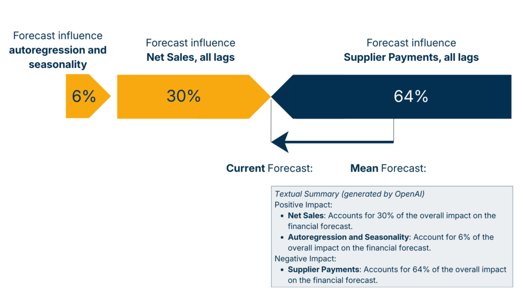
SHAP-based decomposition of a time series forecast showing the contribution of Net Sales (target variable), Supplier Payments (exogenous feature), and autoregressive seasonal effects.
Forecast revisions are the most common point where trust is either gained or lost. Why does a forecast change between two points in time even though it refers to the same month?
Two typical questions arise:
The methodological principle is straightforward:
Forecasts can change between runs for clearly identifiable reasons:
This causal logic is important because it structures discussions: a revision is not “unexplainable” but can be traced back to concrete changes.
Explainability is only effective if it remains usable in operational environments.
Important practical aspects include:
Explainable AI in time series forecasting is methodologically well understood. However, practical implementation reveals several structural challenges.
Standard libraries exist for calculating SHAP values. However, in their default form they are not specifically designed for time series models.
Time series models typically include:
Applying standard SHAP implementations directly often results in explanations that are mathematically correct but poorly aligned with time series structures.
Therefore, explainable time series forecasting requires adapted visualization and aggregation approaches, particularly for lag-based effects.
In practice, it becomes clear that integrating Explainable AI into an existing forecasting system at a later stage can require significant implementation effort.
SHAP calculations must:
Experience shows that considering explainability early in the system architecture is significantly easier than integrating it later.
Explainability is not purely a technical problem.
Even if SHAP values are calculated correctly, this does not automatically mean that the explanations are understood or accepted.
In practice, close collaboration with business users is necessary to:
Explanations are only used when they match the actual information needs of the target audience.
Forecasting systems are not only evaluated based on whether they produce predictions. They are evaluated based on whether those predictions are understood and used.
SHAP provides a methodological foundation for explaining forecast drivers as additive contributions. However, the real value emerges when explaining revisions:
Forecast revisions become explainable when the SHAP values of two predictions are compared.
The central thesis is therefore:
A forecasting system does not become trustworthy through more complex models, but through explainable revisions.
Explainable time series forecasts provide not only a forecast value but also transparent drivers that explain what influences a prediction and what causes changes between forecasting runs.
SHAP values are based on Shapley values from game theory and distribute a prediction fairly across the underlying influencing factors within an additive explanation model.
The sum of SHAP values equals the difference between the current prediction and the average prediction. This allows a forecast to be represented as a baseline plus contribution effects.
By subtracting the SHAP values of the two predictions from each other.
Typical causes include new target values, new or updated indicator values, and model changes such as parameters, indicators, or algorithms.
Complexity reduction is essential to ensure that explanations remain usable for business users.
For some business users, textual explanations are important because they allow forecasts to be explained internally.